Load Derivation for Two Addressing Schemes in a Tree Node Network
1. Definition
Consider a perfect (x)-ary tree-structured network with depth (h), and denote the root node by (a).
The second-level nodes are:
$$ a.a,\ a.b,\ \dots,\ a.x $$
The third-level nodes are:
$$ a.a.a,\ a.a.b,\ \dots $$
Each node is a server that provides identifier resolution service for the subtree rooted at itself. e.g.:
$$ a.b/test $$
This denotes a request for data under node (a.b).
1.1 Constraint
Each node is derived from its parent node. e.g.:
a.b.c is derived from a.b
a.b is derived from a
Under this assumption, the client cannot resolve (a.b.c) directly from (a). Instead, during resolution, (a) returns a referral to (a.b), and the client continues the lookup from (a.b).
Note: although the separator . makes the identifier look hierarchical, this is not necessarily true in the real Handle System, whose identifier space is flatter. For example, (a.b.c) may be derived directly from (a). In this article, we only consider the hierarchical case.
Initially, the client only knows the IP address of the root node (a). When the client accesses a new target node, it selects an available resolution entry point based on its local cache. After each successful access to an unknown node, the client caches the IP address of that target node.
1.2 Schemes
Scheme 1: upward propagation of subtree information
Each node knows the addresses of all descendant nodes in its own subtree and propagates this information to its parent. Therefore, if the client has cached an ancestor of the target node, it can query that ancestor directly and obtain the target address in one step. This strategy can be understood as an LCA-based longest-prefix-hit strategy.
Scheme 2: root registration with parent-only local knowledge
Each node registers its own address only with the root, while non-root nodes only know their direct children. If the client has cached the direct parent of the target node, it queries that parent; otherwise, it queries the root node (a).
1.3 Divergence
Intuitively, both schemes can achieve constant-level resolution hops for a single lookup. The key difference is not the total number of requests, but where the resolution and update load is placed:
Scheme 1 reduces root read load, but introduces update amplification: a node update must be propagated to all ancestors.
Scheme 2 has higher root read load, but lower update propagation cost.
2. 树规模
完美 (x) 叉树,深度为 (h),根深度为 0,叶子深度为 (h)。
总节点数:
$$ N = \sum_{i=0}^{h} x^i = \frac{x^{h+1}-1}{x-1} $$
叶子节点数:
$$ L = x^h $$
内部节点数:
$$ I = N - L = \frac{x^h-1}{x-1} $$
当 (h) 较大时:
$$ \frac{I}{N} \approx \frac{1}{x} $$
$$ \frac{L}{N} \approx \frac{x-1}{x} $$
也就是说,随机访问一个节点时,大部分节点其实是叶子节点,内部节点只占约 (1/x)。
这个事实会解释为什么方案二中的 (x) 会被抵消。
3. 缓存模型
先分析单个客户端。
设客户端已经缓存了 (t) 个不同节点,缓存集合记为:
$$ S $$
其中:
$$ |S| = t $$
先采用一个简化模型:这 (t) 个缓存节点可以近似看作从全网 (N) 个节点中均匀随机抽出的 (t) 个节点。
因此,对于任意一个固定节点 (u),它在缓存中的概率是:
$$ P(u \in S) = \frac{t}{N} $$
这个结论非常重要。
它不是因为 (u) 是内部节点或叶子节点,而是因为缓存是从全部 (N) 个节点中抽取的。对任何一个固定节点来说,被抽中的概率都是:
$$ \frac{\text{缓存大小}}{\text{总节点数}} = \frac{t}{N} $$
4. 方案二:父节点命中模型
方案二中,目标节点 (v) 可以绕过根,当且仅当:
$$ parent(v) \in S $$
也就是说,客户端已经知道目标节点的直接父节点。
对于一个随机目标节点 (v),它的父节点是某个固定内部节点。由于任意固定节点在缓存中的概率都是 (t/N),所以:
$$ P(parent(v) \in S) = \frac{t}{N} $$
因此,方案二的免根概率是:
$$ P_{\text{hit}}^{(2)}(t) = \frac{t}{N} $$
根节点被访问的概率是:
$$ P_{\text{root}}^{(2)}(t) = 1 - \frac{t}{N} $$
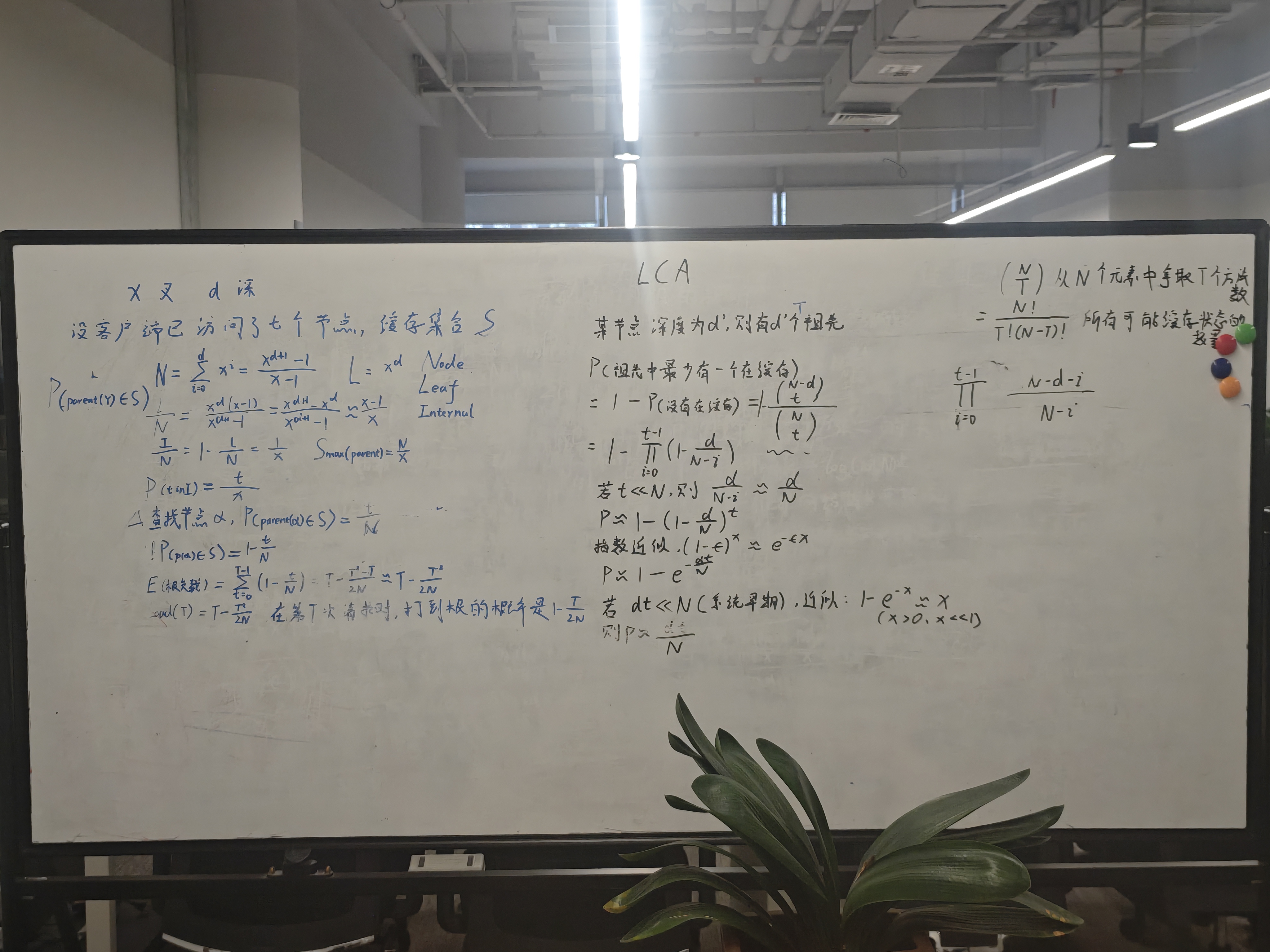
这就是白板左侧的核心公式。
4.1 为什么不是 (\frac{tx}{N})?
直觉上,已知 (t) 个节点,每个节点最多有 (x) 个孩子,所以似乎最多有 (tx) 个节点可以绕过根。
这个上界没错,但它不是期望值。
原因是:缓存中的大多数节点是叶子,叶子没有孩子。
缓存中内部节点的期望数量是:
$$ t \cdot \frac{I}{N} \approx t \cdot \frac{1}{x}
\frac{t}{x} $$
每个内部节点有 (x) 个孩子,所以它们合计覆盖的孩子数量期望是:
$$ \frac{t}{x} \cdot x = t $$
所以真正的免根候选数量期望是 (t),不是 (tx)。
因此:
$$ P_{\text{hit}}^{(2)}(t) \approx \frac{t}{N} $$
这里的 (x) 被内部节点比例 (1/x) 抵消了。
4.2 方案二的累计根负载
如果近似认为每次请求都会带来一个新的缓存节点,那么第 (s) 次请求前,缓存大小约为 (s)。
第 (s) 次请求访问根的概率是:
$$ 1 - \frac{s}{N} $$
那么前 (T) 次请求的累计根访问次数期望为:
$$ R_2(T) = \sum_{s=0}^{T-1} \left( 1-\frac{s}{N} \right) $$
拆开:
$$ R_2(T) = \sum_{s=0}^{T-1}1
\frac{1}{N} \sum_{s=0}^{T-1}s $$
第一项:
$$ \sum_{s=0}^{T-1}1 = T $$
第二项:
$$ \sum_{s=0}^{T-1}s = \frac{T(T-1)}{2} $$
所以:
$$ R_2(T) = T
\frac{T(T-1)}{2N} $$
当 (T) 较大时,可以近似写成:
$$ R_2(T) \approx T
\frac{T^2}{2N} $$
平均根负载比例为:
$$ \frac{R_2(T)}{T}
1
\frac{T-1}{2N} \approx 1-\frac{T}{2N} $$
注意,这个比例是“累计平均比例”,不是瞬时概率。
瞬时根访问概率是:
$$ P_{\text{root}}^{(2)}(T) = 1-\frac{T}{N} $$
5. 方案一:LCA / 祖先命中模型
方案一中,每个节点知道自己整个子树内的所有地址。
因此,如果客户端缓存中有目标节点 (v) 的某个祖先节点,那么客户端可以问这个祖先节点,由它直接返回目标地址。
所以方案一绕过根的条件是:
$$ S \cap Ancestor(v) \neq \varnothing $$
其中 (Ancestor(v)) 表示目标节点 (v) 的可用祖先集合。
如果目标节点深度为 (d),那么它路径上的祖先数量与 (d) 成正比。为了避免根节点本身带来的歧义,我们定义:
$$ \ell(v) = \text{目标节点路径上可用于绕过根的缓存前缀数量} $$
在白板推导里,可以近似把:
$$ \ell(v) \approx d $$
理解为:深度越深,路径上可能命中的前缀节点越多。
5.1 固定目标节点的精确命中概率
固定一个目标节点 (v),假设它有 (\ell) 个可用祖先节点。
缓存大小为 (t)。
我们要求:
$$ P(\text{缓存中至少有一个祖先}) $$
用补集更简单。
“至少有一个祖先在缓存中”的反面是:
$$ \text{没有任何祖先在缓存中} $$
总缓存选法数是:
$$ \binom{N}{t} $$
如果缓存中不能包含这 (\ell) 个祖先,那么只能从剩下的 (N-\ell) 个节点中选 (t) 个:
$$ \binom{N-\ell}{t} $$
所以:
$$ P(\text{没有祖先})
\frac{ \binom{N-\ell}{t} }{ \binom{N}{t} } $$
因此:
$$ P_{\text{hit}}^{(1)}(v)
1
\frac{ \binom{N-\ell}{t} }{ \binom{N}{t} } $$
这是方案一对固定目标节点的精确表达式。
5.2 近似成指数形式
当 (N) 很大,且 (t) 相比 (N) 不太大时,可以近似为:
$$ \frac{ \binom{N-\ell}{t} }{ \binom{N}{t} } \approx \left( 1-\frac{\ell}{N} \right)^t $$
所以:
$$ P_{\text{hit}}^{(1)}(v) \approx 1
\left( 1-\frac{\ell}{N} \right)^t $$
继续使用指数近似:
$$ \left(1-\frac{\ell}{N}\right)^t \approx e^{-\ell t/N} $$
于是:
$$ P_{\text{hit}}^{(1)}(v) \approx 1-e^{-\ell t/N} $$
当 (\ell t/N \ll 1) 时,再用一阶近似:
$$ e^{-\ell t/N} \approx 1-\frac{\ell t}{N} $$
所以:
$$ P_{\text{hit}}^{(1)}(v) \approx \frac{\ell t}{N} $$
这就是白板右侧的核心近似:
$$ P_{\text{hit}}^{(1)} \approx \frac{d t}{N} $$
它的含义是:
方案一中,一个缓存节点不只覆盖自己的直接孩子,而是可能通过祖先路径覆盖更深的子树。因此命中概率比方案二多了一个“路径长度因子”。
6. 对所有目标节点取平均
不同目标节点的深度不同,所以 (\ell(v)) 不同。
深度为 (k) 的节点数量是:
$$ x^k $$
因此随机访问一个节点时,目标深度的平均值是:
$$ \mathbb{E}[d]
\frac{ \sum_{k=0}^{h} kx^k }{ \sum_{k=0}^{h} x^k } $$
也就是:
$$ \mathbb{E}[d]
\frac{ \sum_{k=0}^{h} kx^k }{N} $$
当 (h) 较大时,由于树的底层节点最多,平均深度接近叶子深度:
$$ \mathbb{E}[d] \approx h - \frac{1}{x-1} $$
所以粗略地可以写成:
$$ \mathbb{E}[d] \sim h $$
而:
$$ h \sim \log_x N $$
因此方案一相比方案二,多了一个大约为:
$$ \log_x N $$
的缓存命中加速因子。
7. 两种方案的根负载曲线比较
7.1 方案二
方案二只利用父节点缓存。
瞬时根访问概率:
$$ P_{\text{root}}^{(2)}(t) = 1-\frac{t}{N} $$
累计根负载:
$$ R_2(T) = T
\frac{T(T-1)}{2N} $$
早期近似:
$$ R_2(T) \approx T-\frac{T^2}{2N} $$
7.2 方案一
方案一利用祖先 / LCA 前缀缓存。
对固定深度为 (d) 的目标:
$$ P_{\text{root}}^{(1)}(d,t) \approx e^{-dt/N} $$
对所有节点平均:
$$ P_{\text{root}}^{(1)}(t) \approx \mathbb{E}_{d} \left[ e^{-dt/N} \right] $$
在粗略近似下,用平均深度代替 (d):
$$ P_{\text{root}}^{(1)}(t) \approx e^{-\mathbb{E}[d]t/N} $$
由于:
$$ \mathbb{E}[d] \sim \log_x N $$
所以:
$$ P_{\text{root}}^{(1)}(t) \approx e^{-t\log_x N/N} $$
8. 核心对比
方案二:
$$ P_{\text{root}}^{(2)}(t) \approx e^{-t/N} $$
方案一:
$$ P_{\text{root}}^{(1)}(t) \approx e^{-t\log_x N/N} $$
所以方案一的根负载下降速度大约比方案二快:
$$ \log_x N $$
倍。
换句话说:
- 方案二需要缓存规模达到 (O(N)),根负载才会显著下降;
- 方案一大约只需要缓存规模达到:
$$ O\left(\frac{N}{\log_x N}\right) $$
根负载就会明显下降。
这就是方案一的数学优势。
9. 但是方案一的存储成本更高
方案一中,每个节点保存自己整个子树的信息。
一个节点的地址会被它所有祖先保存一次。因此总存储量等价于:
$$ \sum_{\text{所有节点 } v} depth(v) $$
也就是:
$$ \sum_{k=0}^{h} kx^k $$
因此:
$$ Storage_1 = O(Nh) $$
因为:
$$ h = \log_x N $$
所以:
$$ Storage_1 = O(N\log_x N) $$
方案二中:
- 根保存全局 (N) 个地址;
- 每个非根内部节点只保存直接孩子;
- 总体仍是线性级别。
因此:
$$ Storage_2 = O(N) $$
10. Read-Write Trade-off
10. 总请求数是否相同?
如果目标节点尚未被客户端直接缓存,那么两种方案都可以做到:
$$ \text{解析入口} \rightarrow \text{目标节点} $$
也就是常数级解析。
所以从“总请求跳数”看,两者差异不大。
真正的区别在于:
$$ \textbf{解析请求打到哪里} $$
方案二中,大量解析请求早期会集中到根。
方案一中,解析请求会更快被分散到树中的各级祖先节点。
因此:
| 指标 | 方案一:LCA / 子树递推 | 方案二:父节点 / 根注册 |
|---|---|---|
| 单次定位跳数 | 常数级 | 常数级 |
| 根负载下降速度 | 快,约 (e^{-t\log_x N/N}) | 慢,约 (e^{-t/N}) |
| 收敛缓存规模 | (O(N/\log_x N)) | (O(N)) |
| 存储开销 | (O(N\log_x N)) | (O(N)) |
| 本质 | 用存储换根负载分散 | 用根中心化换低存储 |
11. 结论
方案一和方案二的核心差异不是“能不能一跳定位”。在你的设定下,两者都可以做到常数级定位。
真正差异是:
$$ \textbf{缓存命中可以覆盖多少潜在目标} $$
方案二中,一个缓存节点主要帮助它的直接孩子,因此命中增长速度是:
$$ \frac{t}{N} $$
方案一中,一个缓存节点如果是目标路径上的祖先,就可以帮助整个子树,因此命中增长速度带有路径长度因子:
$$ \frac{dt}{N} $$
对整棵树平均后,这个因子约为:
$$ \log_x N $$
所以方案一用更高的状态复制成本,换来了更快的根负载下降。
最终可以概括为:
$$ \boxed{ \text{方案一:空间换根负载} } $$
$$ \boxed{ \text{方案二:低存储但根负载收敛慢} } $$
后续如果加入非均匀访问,方案二会因为热点父节点更快进入缓存而改善;如果加入节点信息变更噪声,方案一会因为上推状态更多而面临更高的失效传播成本。这两个因素会改变最终的工程取舍。